The Math behind DSF SynthesisIntroductionDiscrete Summation Formulae (DSF) Synthesis, which has been used in all Moppelsynths so far to achieve maximum signal quality, is a synthesis technique that computes a bandlimited, harmonic signal. The generated timbres are quite similar to those of FM synthesis, yet DSF Synthesis doesn't require oversampling and filtering since it can compute directly only the desired harmonics below the Nyquist frequency. Owing to this, the generated signal is of high quality, free of aliasing artefacts and phase distortion.However, the quality comes at the price of a bit more CPU-intensity and not-so-trivial theory and implementation. Seeing how people get all orgasmic about VST synths with squashed sound with a reverb on top, you may want to ponder if it's worth the effort. This article describes how to derive the formulas of DSF Synthesis. At the same time, it explains a DSF variant that has been used in the Tetra and Sonitarium synths and that is more general than the one proposed by Moorer in that it generates an additional series of cosines to obtain a quadrature signal, a stereo signal whose harmonics are pairwise out of phase by 90 degrees. In between, a simple introduction to sine and cosine calculation by complex numbers is provided. The ObjectiveTo generate harmonic sound, a synthesis technique must generate a series of sinusoids such that the frequency difference between two neighbored sines is everywhere the same. In the digital sound synthesis domain, DSF Synthesis attempts to achieve that in a straightforward manner by fast calculations of formulas of the form
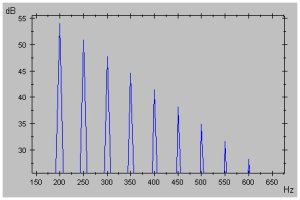
There are N+1 partials, the fundamental is fc, the distance between two subsequent harmonics is fm, and the harmonics' magnitudes fall off by factor w. On a decibel scale, the partials fall off linearly.
Computing all those sines would be quite slow, though, and DSF Synthesis fixes that by computing an equivalent formula that doesn't make it necessary to sum up all the sines. This means it aims for nothing less than generating a bandlimited signal without adding all sines separately (unlike Additive Synthesis), and without having to oversample and filtering out the harmonics above the Nyquist frequency (unlike Frequency- or Phase-Modulation Synthesis have to do). So, how does DSF Synthesis do that? Sines and Cosines by Phasor RotationsIn order to understand the math behind DSF synthesis, we first have to examine what sines and cosines are all about. Suppose we have an arc rotating counter clockwise around the center of the Cartesian coordinate system in a plane. If that so-called phasor has length A and rotates by an angle of w per second, then after t seconds the x-coordinate of the tip of the phasor is A*cos(w*t) and the y-coordinate is A*sin(w*t): Sines and Cosines by Complex Number MultiplicationsIn fact, such phasors can be described conveniently by complex numbers such that a rotation can be performed with a couple of simple arithmetic operations. Complex numbers can be viewed as ordered pairs [a,b] or as points in the plane for which addition, subtraction, multiplication and division are defined so we can calculate with them just like with real numbers. The x-coordinate of a complex number is commonly called its real part and its y-coordinate is called its imaginary part. To denote the real and imaginary parts of a complex number, we define:RE([a,b]) = a and IM([a,b]) = b Addition and subtraction of two complex numbers are simply defined like this: [a1,b1] + [a2,b2] = [a1+a2, b1+b2] [a1,b1] - [a2,b2] = [a1-a2, b1-b2] The multiplication is defined like this: [a1,b1] * [a2,b2] = [a1*a2 - b1*b2, a1*b2 + b1*a2] The division is somewhat more complicated and defined like this: [a1,b1] / [a2,b2] = [(a1*a2 + b1*b2) / (a2*a2 + b2*b2), (b1*a2 - a1*b2) / (a2*a2 + b2*b2)] Notice that the real numbers can be viewed as the subset of the complex numbers in that they can be represented by complex numbers with imaginary component 0: a1 + a2 = [a1,0] + [a2,0] = [a1+a2,0] a1 * a2 = [a1,0] * [a2,0] = [a1*a2 - 0*0, a1*0 + 0*a2] = [a1*a2,0] and x * [a,b] = [x,0] * [a,b] = [x*a, x*b]. Also notice that every complex number can be viewed as an arc and vice versa. That is, for each complex number [a1,b1] there exists an A and an angle w such that: [a1,b1] = A * [cos(w),sin(w)], where A is the length of the arc described by [a1,b1]. One feature of complex numbers that is particularly valuable for sound synthesis is that you can use them easily to implement rotating phasors by complex number multiplications, because it can be shown that (A*[cos(w),sin(w)]) * (B* [cos(g),sin(g)]) = A*B * [cos(w+g),sin(w+g)] That means, we can rotate a complex number by the angle w by multiplying it with the complex number [cos(w),sin(w)]. From this observation, we can already derive a simple oscillator that quickly generates both a sine and a cosine wave. For each sample, we just have to perform a complex multiplication of a phasor with a suitable complex number of the form [cos(w),sin(w)]. Every now and then, we have to normalize the phasor, ie. reset it to length 1. Because, otherwise, by the roundoff errors introduced by the arithmetic operations, it will not keep the legnth 1 but degenerate. When using double precision floating point variables, this normalization needs to be done only occasionally, eg. every few thousands of samples.
This is just to get a rough idea how complex number arithmetic can be used for synthesis. But complex numbers can do much more, they can help us compute the DSF formula. Deriving the Classic DSF FormulaWe will now examine how to rewrite the target formulas(t) = ∑k=0..N wk sin(2p(fc + k fm) t / sampletime) by the help of complex numbers such that we get a closed-form expression, ie. the sum will vanish (and by that, there will be no need to sum up all the sines when computing the samples). In fact, we can calculate s(t) by calculating the following complex formula: c(t) = ∑k=0..N a * bk, where
Anyway, s(t) can be easily obtained from c(t) since it is true that s(t) = IM(c(t)), which means that we can obtain s(t) by picking the second number from each sample couple generated by c(t). To see that s(t) = IM(c(t)), please observe that c(t) = ∑k=0..N a * bk = ∑k=0..N [cos(2p fc t / sampletime), sin(2p fc t / sampletime)] * [w*cos(2p fm t / sampletime), w*sin(2p fm t / sampletime)]k = ∑k=0..N [cos(2p fc t / sampletime), sin(2p fc t / sampletime)] *[wk *cos(k * 2p fm t / sampletime), wk *sin(k * 2p fm t / sampletime)] = ∑k=0..N [wk cos(2p(fc + k fm) t / sampletime), wk sin(2p(fc + k fm) t / sampletime)] = [∑k=0..N wk cos(2p(fc + k fm) t / sampletime), ∑k=0..N wk sin(2p(fc + k fm) t / sampletime)] So we can get s(t) by computing c(t) and picking its imaginary part. c(t), again, resembles a prominent geometric series and can be simplified on complex numbers just like it's done on real numbers: c(t) = ∑k=0..N a * bk = a * (1 - bN+1) / (1 -b) Woosh, the sum is gone! So we can simplify s(t) like this: s(t) = IM( c(t) ) = IM( a * (1 - bN+1) / (1 -b)) which is, since IM(x*y) = RE(x)*IM(y)+IM(x)*RE(y) (this follows from the definition of complex multiplication) = RE(a)*IM((1 - bN+1) / (1 - b)) + IM(a)*RE((1 - bN+1) / (1 - b)) which is, since RE(x/y) = (RE(x)*RE(y)+(IM(x)*IM(y)) / (RE(y)*RE(y)+IM(y)*IM(y)) and IM(x/y) = (IM(x)*RE(y)-RE(x)*IM(y)) / (RE(y)*RE(y)+IM(y)*IM(y)) = ( RE(a)*(IM(1-bN+1)*RE(1-b)-RE(1-bN+1)*IM(1-b)) + IM(a)*(RE(1-bN+1)*RE(1-b)+IM(1-bN+1)*IM(1-b)) ) / (RE(1-b)*RE(1-b)+IM(1-b)*IM(1-b)) = ( cos(u)*((-wN+1*sin((N+1)*v))*(1-w*cos(v))+(1-wN+1*cos((N+1)*v))*w*sin(v)) + sin(u)*((1-wN+1*cos((N+1)*v))*(1-w*cos(v))+wN+1*sin((N+1)*v)*w*sin(v)) ) / ((1-w*cos(v))2+(w*sin(v))2) where u = 2p fc t / sampletime and v = 2p fm t / sampletime. Applying further transformations by trigonometric formulas, this becomes after a while: = { ( w*sin(v-u) + sin(u) ) + wN+1* (w* sin(u + N*v) - sin(u + (N+1)*v)) } / ( 1 + w2- 2*w*cos(v) ) That's it! In summary, we have just derived the classic DSF formula proposed by Moorer, which is
Classic DSF Synthesis vs. Complex DSF SynthesisActually, we have just derived two methods to perform DSF Synthesis. On the one hand, we can use the classic DSF formula to computes(t) = ∑k=0..N wk sin(2p(fc + k fm) t / sampletime). On the other hand, why not compute the complex formula c(t) instead of s(t), using complex arithmetic? After all, computing the complex c(t) samples will give us two samples with each sample step, which can be used for stereo output. As shown before, we have c(t) = ∑k=0..N [cos(u), sin(u)] * [w*cos(v), w*sin(v)]k = [∑k=0..N wk cos(u + k*v), ∑k=0..N wk sin(u + k*v)] where where u = 2p fc t / sampletime and v = 2p fm t / sampletime. So computing c(t) gives us a complex signal, the imaginary part of which is the sum of sines like it is obtained by classic DSF Synthesis, and the real part of which is a sum of cosines. Sending one signal to the left stereo channel and the other to the right channel, we get a quadrature stereo signal, ie. the harmonics of the signal are pairwise out of phase by 90 degrees (since cos(x) = sin(90° - x)).
This is the synthesis technique used in Tetra and Sonitarium. The computation can be made much faster if the expensive sin and cos functions are not called during each sample step but only when a new key is pressed. At that time, phasors can be initialized by using the standard sin and cos functions, and after that, rotating phasors can be used for fast sine and cosine calculation, as has been described before for the simple osciallator example. This optimization is used in Sonitarium. By the way, when using the formulas presented so far, the harmonics will fall off to the right side of the fundamental. If you want them to fall off to the left side, just let the complex result of the expression "(1 - [w*cos(v), w*sin(v)]N+1)/(1 - [w*cos(v), w*sin(v)])" be computed as usual, then flip the sign of its imaginary part. This way you will get another complex signal by a simple sign flip. You can then mix it with the first signal or whatever. NormalizationOn issue not mentioned yet is the normalization of the signal. After all, the signal would get much too loud with all those sines and cosines summed up. A simple estimation that has proven useful for both classic and complex DSF synthesis is that the volume of the computed signal is at most∑k=0..N wk, which is equal to (1 - wN+1)/(1-w), where w is the weight factor of the harmonics. Divide each sample by that value, and you're done. Thanks for reading, Burkhard (moppelsynths@verklagekasper.de) Literature
James
A. Moorer, "The
Synthesis of Complex Audio Spectra by Means of Discrete Summation
Formulas", http://www.jamminpower.com/main/articles.html,
1976. |
Back to "Moppelsynths"